

ABSTRACT: There is an avoidable tension in a recently presented argument against the income effect from the perspective of Austrian or causal-realist price theory. The argument holds that a constant purchasing power of money is a necessary assumption for constructing an individual demand curve for a specific good, and hence that price changes along the demand curve are by definition incapable of exerting a “purchasing power effect,” that is, an income effect in standard neoclassical terminology. Price changes are, however, never neutral to the purchasing power of money. We show that the necessary assumption for the construction of a demand curve for a specific good is not the constant purchasing power of money as such, but rather constant opportunity costs of expending money on the good in question. On this basis we show that it is possible to derive a type of income effect in causal-realist price theory. Yet, it might be more appropriate to call it a “wealth effect.” Regardless of important and undeniable differences, the gulf between neoclassical and Austrian microeconomics on this point is thus smaller than it has been made to be.
KEYWORDS: income effect, wealth effect, causal-realist tradition, price theory, demand theory
JEL CLASSIFICATION: B53, D11
Karl-Friedrich Israel (Kf_israel@gmx.de) is lecturer at the Institute for Economic Policy at Leipzig University, Germany.
Quarterly Journal of Austrian Economics 21, no. 4 (Winter 2018) full issue, click here.
1. INTRODUCTION
In a recent publication, Salerno (2018) argues that the income effect is an illusion of neoclassical microeconomics. He demonstrates his claim on the basis of causal-realist price theory in the tradition of Menger, Böhm-Bawerk, Mises, Robbins, Wicksteed, and Rothbard. He thereby picks up a long-standing debate that emerged with Friedman (1949, 1954), who questioned the Hicksian interpretation of the Marshallian demand curve that became the standard view in modern microeconomic demand theory.
Moreover, Salerno rebuts a critique raised by Caplan (1999) against Rothbard (2009 [1962]). The latter was accused of contradicting himself when he rejected the idea of the income effect, while still considering backward-bending labor supply curves to be possible. In fact, Salerno demonstrates that a backward-bending labor supply curve can be derived simply from the law of marginal utility and a given value scale on which leisure is ranked against money balances. Hence, the backward-bending labor supply curve is in principle independent of the income effect as explained in standard neoclassical micro.
While the gist of Salerno’s argument is sound, there is a certain tension related to the ceteris paribus assumptions he invokes. A slight adjustment of the assumptions, however, suggests that there is a type of income effect to be identified in causal-realist price theory. A more appropriate label might be “wealth-effect,” since what matters in causal-realist demand and price theory are stocks of goods that individuals possess and demand at any given moment, rather than flows of goods, which are a derivative of exchanges, as Salerno convincingly argues.
We will first summarize Salerno’s argument in the next section before the tension caused by his stated assumptions is highlighted. We will then proceed to conduct a similar analysis with an adjusted set of assumptions. Finally, the income or “wealth” effect that emerges is illustrated by means of a numerical example.
2. THE CAUSAL-REALIST ARGUMENT AGAINST THE INCOME EFFECT
Standard neoclassical microeconomics separates the effect of price changes along a given demand curve into substitution and income effects. This analysis was introduced by Hicks (1946 [1939]). The underlying assumptions for the construction of the demand curve for a certain good are that the actor’s tastes and preferences, their monetary income, as well as the money prices of all other goods remain constant. Hence, a change of the money price for the good under consideration along the demand curve has an impact on real income and the corresponding budget constraint.
Since then, the income effect has enjoyed a long-lasting but scattered debate in neoclassical microeconomics as summarized by Salerno (2018, pp. 27–30). He argues that Friedman and his followers were adopting a specific set of assumptions for positivist reasons. These assumptions would rule out an income effect.1 The Friedmanite income-compensated demand curve would facilitate the formulation of empirically testable predictions. Salerno thus closely follows Yeager’s (1960) review of the Methodenstreit over demand curves.
In contrast, the causal-realist rejection of the neoclassical income effect is not based on these positivist considerations that motivated Chicago School economists. Salerno attempts to show that the causal-realist rejection is at least implicitly contained, for example, in the writings of Wicksteed (1933), Mises (1998 [1949]) and Rothbard (2009 [1962]) (see also Salerno 2011, p. 14), and that it can be logically justified as an implication of the existence of value scales and the law of diminishing marginal utility.2
Demand curves in that tradition are taken to be pedagogical tools used to illustrate the inverse relationship between the money price of any good and the quantity demanded, which is an essential part of the process of market price formation. Demand curves are thus not seen to be “real” or anything measurable and observable in the external world. They are abstractions from subjective ordinal preference rankings, which are more fundamental and in an important sense “real,” as they partly reveal themselves in every action and choice: “Without the concept of a scale of values, it would be impossible to even describe an acting being or speculate meaningfully about the subjective processes that give rise to purposeful behavior” (Salerno 2018, p. 31).
Different individual value scales in combination with the existing stocks of goods owned by those individuals determine the equilibrium structure of quantities and prices of goods exchanged on the market. As Salerno (2018, p. 31) puts it: “This momentary equilibrium position denotes a state in which all consumers allocate expenditures across goods so that the marginal utility of the last unit of each good purchased just exceeds the marginal utility of the sum of money expended for its price.” Demand and supply curves are just means to facilitate the grasp of that mechanism.
One fundamental distinction from the standard neoclassical view that can be drawn directly from this statement is that money itself is treated as a valuable good in causal-realist analysis. It is not simply taken to be a measure of value, or a numeraire. Another important difference is that income as a flow of money plays only a secondary role. In fact, income is the result of market exchanges at certain money prices that one seeks to explain, but “[a]t the moment before any set of exchanges is consummated all that objectively exists are given individual stocks of goods and money” (p. 32).
Salerno does not deny the indirect impact that expected future income may have on the subjective value of existing cash balances in the present. However, for actual monetary exchanges occurring on the market, it is precisely the latter that is crucial: the subjective valuation of cash balances at the moment immediately before the exchanges are realized.3
In order to derive a demand schedule, certain ceteris paribus assumptions are necessary. According to Salerno (2018, p. 32),
[b]ecause it seeks to explain prices as the outcome of a unitary valuation process that includes money, causal-realist price theory holds the following data constant in deriving the individual demand curve: 1. the buyer’s value scale; 2. his money balances; 3. all other prices; and 4. the (anticipated) purchasing power of money.
Thus, in Salerno’s (2018, p. 34) presentation of the argument, in order to be able to rank units of money along with various units of other goods on an ordinal unitary value scale a given purchasing power of money must be presupposed:
In the causal-realist derivation of the individual demand curve, then, units of various goods and of money are ranked and compared with one another by the individual. But in order to intermingle units of money with units of goods on a unitary value scale and judge their relative utilities, a pre-existing purchasing power of money must be assumed.
This assumption is deemed necessary by Salerno, because one has to “abstract from the complexities of the value scale […] to trace out a curve that isolates the relationship between the price and quantity demanded of a single good” (p. 35). Hence, if variations in the purchasing power are not permissible, when constructing demand curves, there can be no such thing as an “income effect,” which relies on changes in the purchasing power of money. This is why Salerno calls it more appropriately “purchasing power effect.” He summarizes his argument as follows:
Put another way, the demand curve is based on a person’s overall economic position and his expectations prevailing in the moment preceding action […] If this were not the case, if the demand curve did not refer to a period temporally and logically antecedent to action, it would be impossible for individuals to formulate a coherent value scale, because the purchasing power of money would be unknown and units of money could not be meaningfully ranked against units of goods. The very existence of money prices thus logically implies the absence of an income effect or, more properly, a “purchasing power effect.” That is, in causal-realist analysis, the individual’s ex ante real money stock cannot vary with movements along the demand curve, because the curve can only be derived based on an already existing and “known”—or rather, definitely anticipated—purchasing power of money. (Salerno 2018, p. 36)
The effect emerging from a price change along a given demand curve would then have to be interpreted entirely as a substitution effect (Salerno 2018, pp. 36-37).
3. THE TENSION IN THE ARGUMENT
The problem with the argument presented by Salerno (2018) lies in the ceteris paribus assumptions that hold all other prices (3) as well as the purchasing power of money (4) constant, while the price of the good under consideration is allowed to change along the demand curve. If the assumption of a constant purchasing power is really necessary to construct the demand curve in the first place, then an obvious tension emerges once we allow the money price for the good to vary along that curve. Changes of the money price of a good are inextricably linked to the purchasing power of money.
The purchasing power of money corresponds to the array of goods that can be exchanged against a given sum of money on the market. Hence, whenever some money price is allowed to change ceteris paribus, it has a direct effect on the purchasing power of money. When a money price increases along the demand curve, then the exchange value of money and hence its purchasing power decrease, and vice versa. If, however, the demand curve for a specific good is itself contingent on the purchasing power of money, a price change along a given demand curve is contradictory as it destroys the underlying assumption on which the demand curve is based. In other words, a price change along the demand curve affects the demand curve itself as it changes the purchasing power of money. There could thus be no price change along the demand curve.
Salerno (2018, p. 34) himself is aware of the problem to a certain degree, but he seems to be convinced that it is sufficiently mitigated by invoking the time element:
The marginal utilities of goods today are derived directly from the varying importance of the wants they are expected to satisfy today. However, judging the subjective marginal utility of money today necessarily entails knowing yesterday’s objective purchasing power of money, that is, the inverse of the structure of money prices in all their particularity. This means that before an individual can formulate his value scale in anticipation of today’s exchanges, he must refer back to the purchasing power of money that emerged in the immediately previous round of exchanges. In other words, an individual’s value rankings and marginal utilities of goods and money, which are operative in determining today’s structure of prices, are based on today’s valuations of goods and money. But the valuation of money today must refer back to yesterday’s purchasing power of money, because it is the only means by which its prospective purchasing power in today’s market can be anticipated and its marginal utility set. If money did not have a pre-existing purchasing power — that is, if money never exchanged against goods in the past — market participants would lack the knowledge needed to assign a value ranking to it and, consequently, no one would accept it in exchange for goods today. […] Every money price therefore always contains a time component. […]
There is, therefore, no contradiction in assuming that the purchasing power of money is constant and that the price of the good whose demand curve is being analyzed is permitted to vary. For the purchasing power of money that is held constant and on the basis of which the individual establishes his demand curve today is the purchasing power of money expected to prevail today, which refers back to yesterday’s structure of prices as the starting point for the forecast.
This is unconvincing, since the purpose of the whole exercise is to illustrate and “explain the formation of ´realized prices’,” as Salerno (2018, p. 32) pointed out earlier in his article, that is, in other words, the purpose of the exercise is to explain the purchasing power of money, at least partly, with respect to a certain good. If the demand curve derived rests on the assumption that the purchasing power of money remains constant, then it does not give us what it is supposed to, namely, the isolated relationship between the price and quantity demanded of a single good and hence an illustration of an essential part of the price formation process on the market that in turn explains changes in the purchasing power of money.
There is no question about the necessity of ceteris paribus assumptions in order to derive a demand curve from a hypothetical subjective value scale. We obviously have to keep that value scale constant, but the assumptions cannot extend to the phenomena we seek to explain. Fortunately, the problem is easily solved with a slight adjustment of the assumptions.
The demand curve is supposed to give us the quantities of a good that an individual would purchase at different prices. The trade-off that the individual faces is thus between the marginal value of units of money versus the marginal value of units of the good in question. The marginal value of units of money are essentially given by the opportunity costs of expending a given sum of money in exchange for the good in question. These opportunity costs are indeed closely related to the purchasing power of money. More precisely, however, it is the purchasing power of money with respect to other goods that the person values and might want to acquire. There are other factors that might come into play, such as the expectations about the future development of the purchasing power of money, future monetary income etc. Whatever it may be, the important assumption for the construction of a demand curve from an ordinal value scale is that the subjective value of money does not vary relative to the subjective value of the good in question.
Hence, what is needed in order to derive an individual demand curve for a good is simply a fixed ordinal preference ranking of units of money and units of the good. Since, that ranking is subjective and the relative importance of the factors that influence it ultimately is subjective too, we cannot boil this assumption further down. Taking for granted that the only purpose of money is to be exchanged and that its subjective value derives essentially from its purchasing power, we could reformulate the assumption in very much the same way as Hicks did, namely, that money prices for all other goods would have to remain unchanged. Hence, with respect to Salerno’s stated assumptions, there is only a minor adjustment needed. One has to hold constant: 1. the buyer’s value scale; 2. his money balances; 3. all other prices; and 4. the (anticipated) purchasing power of money with respect to other goods.4 However, strictly speaking, what has to be held constant for the construction of the demand schedule are the opportunity costs of expending a given sum of money on the good in question, whatever the influencing factors of this subjective notion may be.
It is important to realize that for the derivation of a demand schedule we cannot use a fixed preference ranking for units of all conceivable goods on a unitary scale, since such a ranking is indeed dependent on the price structure and would be altered by price changes along the demand curve as Salerno (2018, pp. 36–37) explains. Whether or not an agent would rather have the first unit of good A than the first unit of good B depends on the opportunity costs of acquiring them. The latter are most notably determined by their money prices. Hence, starting from a fixed unitary value scale that ranks units of multiple goods as well as money, we cannot derive the demand curve that we set out to construct, namely, one that allows for analyzing price changes along the curve, because again, price changes along the curve would jeopardize the underlying assumption of the fixed unitary preference ranking that was used to construct the curve in the first place.
Instead, we simply need a fixed preference ranking for units of money and units of the one good that we wish to analyze. No other goods appear in the ranking. On such a scale, the changes in the relative ranks of units of the good with respect to units of other goods remain implicit—hidden behind the units of money actually ranked. In fact, this way we could not illustrate substitution effects between different specific goods directly. We can, however, illustrate substitution effects between the one good under consideration and money.
This point deserves emphasis: deriving the demand curve for a good requires fixing its ranks on a unitary value scale. However, changing the money price of the good along the demand curve is not neutral to that ranking, unless the only good against which it is ranked is money. The necessary assumption for such a fixed ranking is that the opportunity costs of expending any given amount of money on the acquisition of the good as well as the subjective value of the good itself remain constant. We can thus analyze the substitution effect between that good and money. The substitution effects with other goods that the latter entails remain implicit. Moreover, it becomes easy to also illustrate a type of income effect, which might rather be referred to as a “wealth effect.”
In fact, as we will show below, the wealth effect is, in a sense, the more fundamental of the two. It is a direct consequence of any price change along the demand curve. A substitution effect only emerges for price changes along a segment of the curve for which the quantity actually changes, and it effectively adds to the wealth effect only in cases where demand is price-elastic.
4. ILLUSTRATION OF THE “WEALTH EFFECT” IN CAUSAL-REALIST PRICE THEORY
The best way to illustrate the above point is to construct a concrete example. We thus imagine a Bavarian farmer who visits the Oktoberfest in Munich, Germany, in order to consume beer.5 He holds a cash balance of €200. The quantity of one-liter units of beer (a Masskrug in German)6 that the farmer consumes, depends on its money price, his subjective valuation of beer, as well as his subjective opportunity costs of expending a given sum of money on beer consumption. All of these factors that we assume for the following analysis to remain constant are captured in the farmer’s ordinal value scale given in Table 1.
Table 1: Ordinal Value Scale of Bavarian Farmer Holding a Cash Balance of €200

This representation of the value scale follows the notation used in Rothbard (2009 [1962]), where the units of the good to be acquired are put in brackets and are ranked amongst the amount of money to be given up in exchange for one unit. From the ranking in Table 1, we can infer that the farmer will always hold on to at least €100 of his initial cash balance of €200, before he consumes the first Masskrug. His reservation price for the first unit of beer is €100. At any price above that threshold, he would abstain from beer consumption entirely. At any price below, he would at least consume one Masskrug. Moreover, he would buy a second unit of beer only at a price below or equal to €40. From the ordinal value scale in Table 1, we can thus derive his entire demand schedule as summarized in Table 2.
Table 2: Bavarian Farmer’s Demand Schedule for Beer Derived From His Ordinal Value Scale
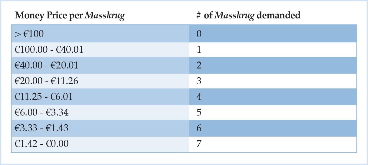
Figure 1: Bavarian Farmer’s Demand Curve for Beer
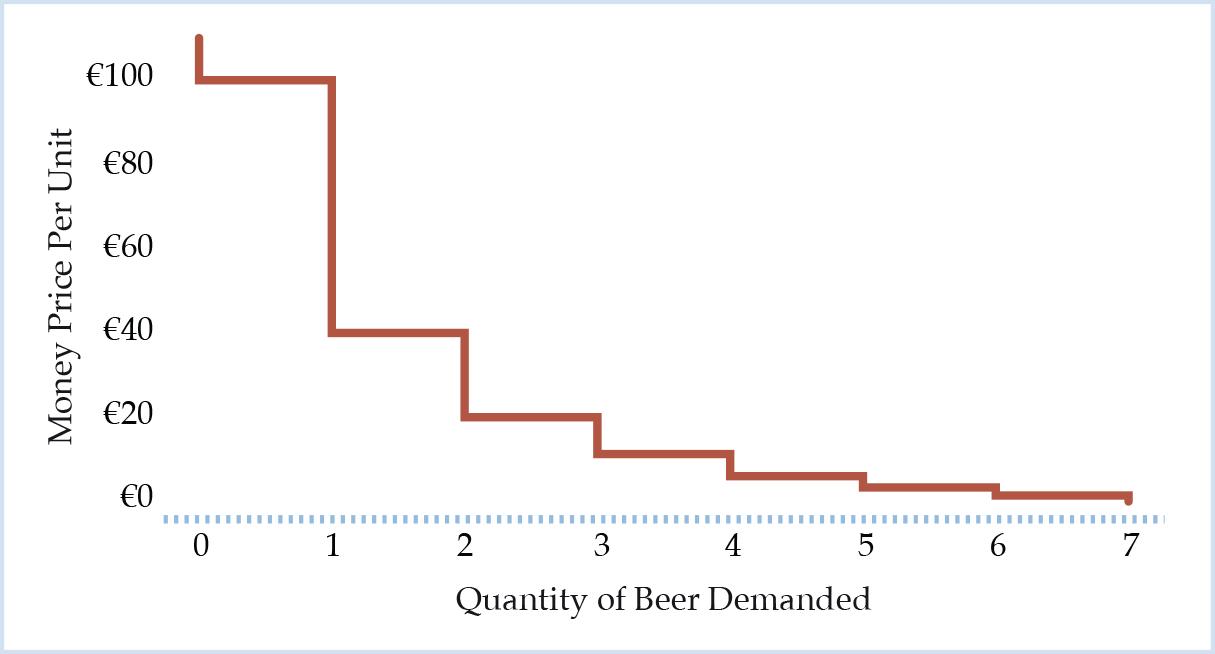
The corresponding demand curve is plotted in Figure 1. As the farmer decides to consume discrete units of beer, his demand curve is a downward-sloping step function.7
Every price-quantity combination along the demand curve for beer corresponds to a certain amount of money that the farmer retains in his cash balance, that is, his retention demand for money. In our analysis, the sum of money retained corresponds to the farmer’s ability to satisfy other wants than his thirst for beer. This includes his demand for other goods that he might also want to consume, such as a roasted chicken, a potato salad, and a good Caribbean cigar, or it might indeed reflect his demand for money as such. The more money he retains, the better he can satisfy his demand for other goods.
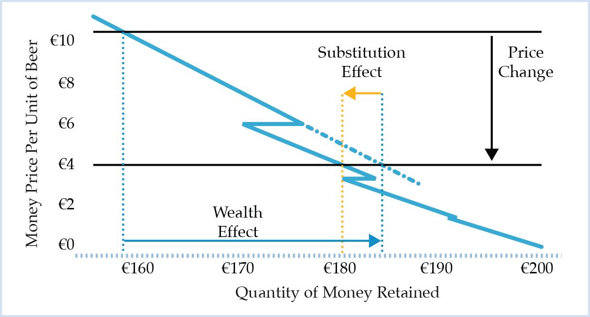
At a price above €100 per Masskrug of beer, the farmer retains his entire cash balance of €200 as his opportunity costs of purchasing beer at the Oktoberfest would be too high. If the price falls below €100, he starts to spend money on beer consumption. He retains 200-P*Q(P) units of money, where P corresponds to the unit price of beer and Q(P) to the quantity of beer demanded at that price. His retention demand for money is plotted in Figure 2. Due to the discrete changes in the quantity of beer consumed, the retention demand for money follows a zigzag pattern.
Figure 2: The Farmer’s Demand for Beer and His Retention Demand for Money as a Function of the Money Price Per Unit of Beer
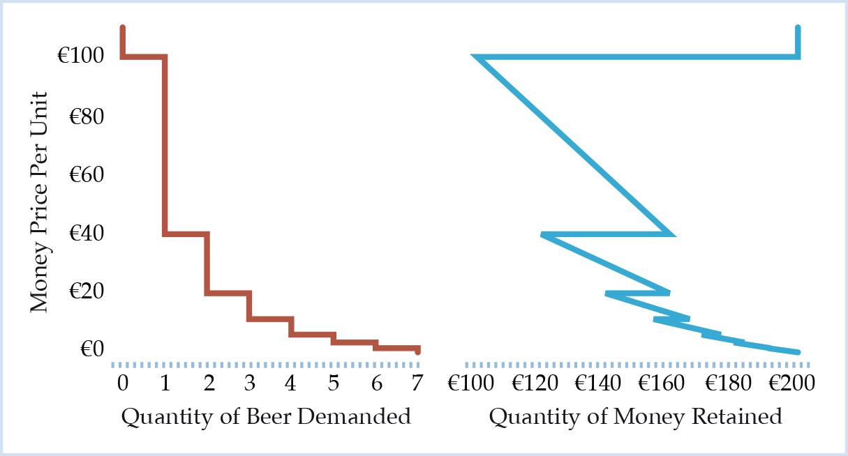
Overall, the retention demand for money increases back to €200 as the price falls from €100 to zero. The zigzag movements of the curve correspond to substitutions between beer and money in the farmer’s cash balance, that is, between beer and any other conceivable good that he might want to acquire with the money retained. When the price falls below a certain threshold, he lowers his retention demand for money in order to increase his demand for beer. For example, as the price falls below €40, the farmer demands a second Masskrug of beer and lowers his cash balance accordingly. He foregoes other ends he might want to pursue with the money in order to consume a larger quantity of beer.
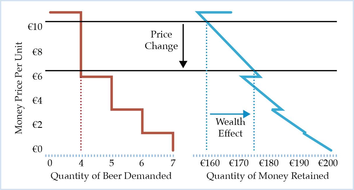
However, the overall trend towards a bigger cash balance retained (over the relevant segment of the curve) as the price for beer decreases, captured in the right panel of Figure 2, also encapsulates a change that can be interpreted as a wealth effect. This wealth effect with respect to the cash balance becomes obvious over any segment of the demand curve for which the discrete quantity of beer consumed remains constant, that is, a segment of the curve for which the price-elasticity of demand is perfectly inelastic. For any such segment, there is nothing but an increase in the cash balance retained as the price for beer decreases and the quantity consumed remains the same. This means that the farmer’s ability to purchase other goods increases while his consumption of beer stays constant. In that sense he becomes wealthier due to decreases of the price for beer along his demand curve.
Figure 3 illustrates this wealth effect with respect to the cash balance as the price per Masskrug of beer decreases from €10.50 to €6.50. The farmer demands four units of beer for any of the two prices, but his cash balance increases from €158 to €174, leaving him better off, that is, wealthier, ceteris paribus, however he decides to use the additional units of money retained.
Figure 3: Illustration of the Wealth Effect with Respect to the Cash Balance as the Price Per Unit of Beer Drops From €10.50 to €6.50
A critic of the above analysis might argue that the example captured in Figure 3 is merely a special case, since the quantity of beer consumed remains constant for the price change under consideration.8 This is certainly true. The example as such does not suffice to show that something akin to the income effect exists in causal-realist price theory. Yet, it already conveys the basic idea. The example can easily be extended to a case where the price-elasticity of demand is not perfectly inelastic and that includes both wealth and substitution effects with respect to the cash balance and their translation into changes in the quantity of beer demanded.
We simply assume a price change from €10.50 to €4.00 as illustrated in Figure 4. Again, at the initial selling price the farmer consumes 4 units of beer and his retained cash balance is €158. At a selling price of €4 per unit he consumes 5 units of beer and the retained cash balance is €180. Both his cash balance and beer consumption have increased. In that sense, he is obviously wealthier than before. There clearly is a wealth effect. Yet, there is also a substitution effect.
The two effects can be separated from each other in the following way. In a first step, we hold beer consumption constant at 4 units. The farmer thus saves €26 because of the price change (4*[10.50 – 4]). His cash balance as a function of the price of beer at constant beer consumption of 4 units is given by the dashed line in Figure 4. It is simply the prolongation of the first segment of the retention demand for money at point (176, 6) under unchanged beer consumption.
Figure 4: Illustration of Wealth and Substitution Effects with Respect to the Retained Cash Balance as the Price Per Unit of Beer Drops from €10.50 to €4.00
In a second step, we adjust the quantity consumed. The cash balance would be €184 without such an adjustment. However, given the value scale of the farmer, we notice that due to the increased cash balance, the marginal value of money has fallen to the point that the farmer would rather substitute another €4 for the fifth unit of beer. This is the substitution effect.
The net effect on the retained quantity of money is an increase by €22, from initially €158 to €180. Solely with regard to the farmer’s retained cash balance the overall effect of the price change along his demand curve for beer consists of a wealth effect of 26€ and a substitution effect of -€4. The substitution can thus be financed entirely out of the farmer’s wealth improvement in terms of his increased cash balance.
In the above example the overall sum of money spent on beer consumption is lower at a unit price of €4 than at a unit price of €10.50. This means that the farmer’s demand for beer is still inelastic, albeit not perfectly inelastic, between the two points considered. However, the same decomposition can be applied to other points on the schedule between which demand is price-elastic, that is, for which the substitution effect outweighs the wealth effect as described above.
Figure 5: Illustration of Wealth and Substitution Effects with Respect to the Retained Cash Balance as the Price Per Unit of Beer Drops from €6.50 to €5.90
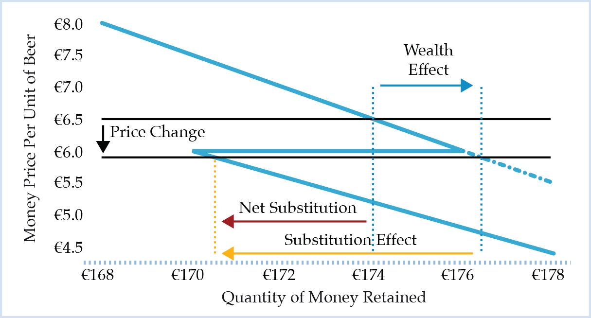
Take, for example, an initial price of €6.50 and an exogenous price drop to €5.90. Analogously to the above case, the wealth effect this time would amount to €2.40 (4*[6.50-5.90]). Without an adjustment of beer consumption, the retained cash balance would thus increase from €174 to €176.40. This would lower the marginal value of money sufficiently to make a substitution of €5.90 for a fifth unit of beer beneficial. The net effect on the farmer’s cash balance is then -€3.50. He ultimately holds a cash balance of €170.50. This case is illustrated in Figure 5.
Only in this last example, for which the demand for beer is price-elastic, that is, the substitution effect outweighs the wealth effect, a net substitution between beer and money occurs. In other words, the increase in beer consumption cannot be financed entirely out of the wealth effect.
In the previous case, shown in Figures 4, the demand for beer is price-inelastic. Hence, there is no sacrifice to be made in terms of a lower cash balance, as compared to the cash balance retained at the initial price, in order to increase beer consumption. There is no net substitution. At the lower price for beer the farmer can increase his beer consumption by one unit and also demand larger quantities of whatever goods happen to have the highest marginal value for him—be that money itself, or any other good he wants to consume. The adjustment in the farmer’s consumption decisions is better interpreted as a pure wealth effect.
In the last example, there is a net substitution. Expansion of beer consumption by one unit as the price falls from €6.50 to €5.90 requires the sacrifice of a diminished cash balance as compared to the cash balance that would have been retained at the higher price. The change in consumption can thus partly be interpreted as a net substitution effect. This, however, does not mean that there is no wealth effect at all. There always is a wealth improvement when the price of one good falls, ceteris paribus, because any basket of goods that could have been acquired without the price change can also be acquired with the price change. Any net substitution must then correspond to a wealth improvement that goes even beyond the wealth effect with respect to the cash balance as described above.
Focusing on the cash balance allows us to express both wealth and substitution effect quantitatively. Only in the case where the substitution effect outweighs the wealth effect, as in Figure 5, a net substitution or sacrifice in terms of a diminished cash balance is necessary to expand the consumption of beer. This means that only a part of the substitution can be financed out of the wealth improvement due to the wealth effect. The remainder of the substitution requires a decrease in the quantity of money retained9 and hence diminishes the farmer’s capacity to acquire other goods.
It is the net substitution with respect to the cash balance that can be interpreted as a genuine (or net) substitution effect with respect to the quantity of beer consumed. The other part, as it is financed out of the wealth effect with respect to the cash balance, can be interpreted as a wealth effect akin to the income effect in standard neoclassical price theory.
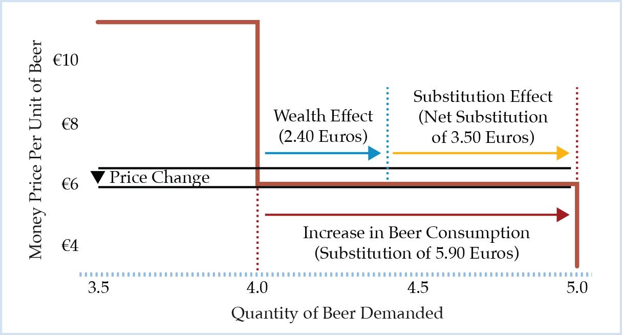
Both effects can be expressed in relative terms. The wealth effect in Figure 5 is €2.40. Hence, 40.68 percent of the increase in beer consumption from the fourth to the fifth unit at a unit price of €5.90 are financed out of the wealth effect, while 59.32 percent of the increase require a net substitution. The net substitution of €3.50 translates into the substitution effect with respect to the quantity of beer. This is illustrated in Figure 6.
Figure 6: Illustration of Wealth and Substitution Effects with Respect to the Quantity of Beer Consumed as the Price Per Unit of Beer Drops from €6.50 to €5.90 and Beer Consumption Increases from Four to Five Units
The proposed decomposition has the following implications. First of all, it allows to quantify the substitution and wealth effects with respect to the retained cash balance in all conceivable cases of an exogenous price change.
When, as a result of a lower unit price, the consumption of beer increases but is price-inelastic (Figure 4), the entire increase in consumption is interpreted as a wealth effect. Since there is no net substitution in such a case, there is no substitution effect with respect to the increased quantity of beer. This is because the cash balance that would have been retained at the higher price is taken to be the relevant benchmark and it is smaller than the cash balance retained at the lower price. Hence, the increase in beer consumption can be financed entirely out of the wealth improvement with respect to the cash balance.
In the case of price-elasticity (Figure 5), there is a net substitution. The cash balance retained at the lower price is smaller than the cash balance that would have been retained at the higher price. Only a part of the increase in beer consumption can be financed out of the wealth effect with respect to the cash balance. This part translates into the wealth effect with respect to beer consumption. The remainder is interpreted as the substitution effect.
The other goods that the farmer might want to acquire remain implicit in the above examples. If we wanted to exemplify the substitution and wealth effects further, we would have to set up a second value scale on which money is ranked against other goods than beer that the farmer wants to purchase at the Oktoberfest.
In order to set up the second value scale, the money prices for these goods have to be held constant.10 From that scale, we could then in very much the same way as above derive the farmer’s demand for other goods as a function of the sum of money he retains after beer consumption. Table 3 contains such a mapping.
Table 3: Bavarian Farmer’s Demand for Other Goods as a Function of the Sum of Money Retained After Beer Consumption Given a Fixed Price Structure for Other Goods (€12 roasted chicken, €6 potato salad, €6 cigar)
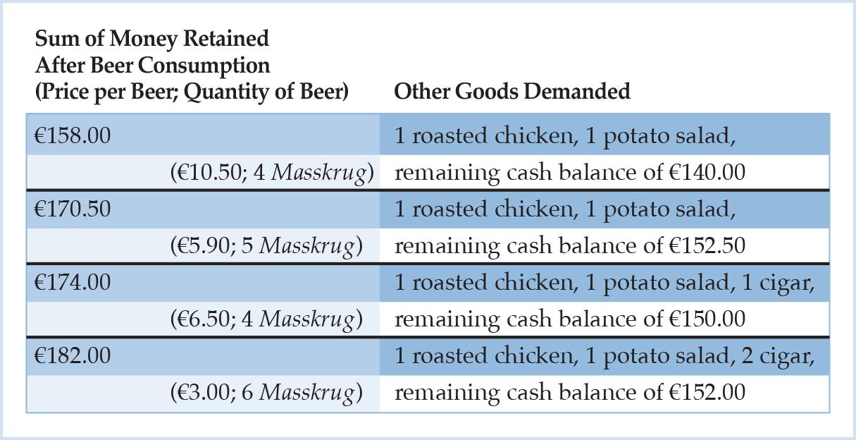
We assume a fixed price structure for the other goods. As the money price for a Masskrug changes along the farmer’s demand schedule for beer, we can now trace the wealth and substitution effects in terms of real consumption decisions. At a price of €10.50 per unit of beer, the farmer retains €158 after beer consumption. However, he decides to also purchase a roasted chicken at €12 and a potato salad at €6, thus reducing his cash balance further to €140. As the price per unit of beer decreases to €6.50, the farmer does not change the quantity of beer consumed, but instead buys an additional supplement rounding up the evening, that is, a cigar for €6. Even though his real consumption increases, his final cash balance is even higher, namely €150, due to the strong decrease in the unit price of beer.
If the unit price was to fall even further to only €3, the farmer would expand his consumption of beer and cigars by one unit each, and still end up with a higher cash balance of €152 at the end. Again, there is no net substitution required.
We can exemplify a net substitution in Table 3 as we imagine again a price change per unit of beer from €6.50 to €5.90. At €6.50, the farmer demands 4 Masskrug and enjoys 1 cigar as a supplement. He holds a final cash balance of €150. At €5.90, however, he would rather drink the fifth Masskrug of beer and forego the enjoyment of the cigar. He would hold a final cash balance of €152.50. He foregoes the consumption of the cigar because the opportunity costs are too high, that is, he prefers to hold a cash balance of at least €146.50 over the consumption of the first cigar. Hence, he substitutes the fifth Masskrug and a slight increase of his cash balance by €2.50 for the first cigar.
We want to emphasize again that there is also a wealth effect associated with the price change from €6.50 to €5.90 per Masskrug of beer. The farmer saves 60 cents on the first four beers he consumes, adding up to an amount of €2.40. This is, taken as such, undoubtedly a wealth improvement. The above approach that takes account of the cash balance allows to give a quantitative expression of the wealth effect. It goes without saying that it does not provide us with an exact measure of the wealth improvement in terms of subjective utility that results from a lower price per unit of beer.
5. CONCLUSION
Salerno (2018) argues that the neoclassical income effect is a theoretical illusion. However, as our analysis has shown, there is a kind of income effect, or rather “wealth effect,” to be identified in causal-realist price theory that plays essentially the same role as the income effect in standard microeconomics. Salerno’s conclusion that everything that emerges from a price change along the demand curve for a specific good are substitution effects, must be regarded as too strong a claim. Salerno is misled by his assumption that the purchasing power of money needs to be held constant in order to derive the demand curve for a certain good.
As seen above, not the purchasing power as such, but the opportunity costs of expending any given amount of money on the good in question need to be held constant. These opportunity costs are undoubtedly related to the purchasing power of money, but it is the purchasing power with respect to all other goods that matters here. If we regard the latter as the only relevant factor, then our assumption for the derivation of the demand curve essentially boils down to Hicks’s original assumption, namely, that the money prices for all other goods have to remain constant. The actual gulf between the standard neoclassical view and the causal-realist or Austrian take on substitution and income effects thus becomes much less pronounced.
However, there are two important points of divergence. First, in the causal-realist tradition, money is treated as an actual good that is valued as such and that is demanded or retained. It is not simply a numeraire. It is through the ordinal ranking of units of money against units of a specific good on a unitary value scale that we can derive the individual demand curve for that good. Second, income plays only an indirect role. The relevant magnitude is the cash balance of an economic actor immediately before exchanges take place. Expected future income may indirectly affect how these cash balances are valued in the present. But the present valuation of the cash balance is decisive, whatever the influencing factors are. Hence, the effect we have illustrated above is more appropriately called wealth effect. It can be given a quantitative expression in terms of changes in the cash balance retained that translates directly into the actor’s capacity to acquire additional goods.
The presented approach provides an easy and direct illustration of a very real phenomenon that most people intuitively understand, namely, that consumers are made better off when a given good can be acquired at a lower money price. The wealth improvement with respect to the cash balance may be used to finance an increase in the quantity of the good demanded. This is the wealth effect. Only the remainder, in case of a price-elastic demand schedule, requires a net substitution. This is the substitution effect.
- 1These assumptions include that real income remains constant, that is, a price change along the demand curve for the good under consideration goes hand in hand with offsetting price changes for other goods (Friedman, 1949, pp. 465–466).
- 2Salin (1996) has previously presented a similar critique of the neoclassical income effect. He concluded that it is a “myth” and since he regarded it as a necessary condition for a backward-bending labor supply curve, he drew the erroneous conclusion that the latter is impossible. Salerno (2018, pp. 37–43) demonstrates why this conclusion is false.
- 3Salerno (2018, p. 32) explains the special role of the concept of income in economic theory as follows:
The notion of (net) income as a “flow” is the outcome of the individual entrepreneur’s judgment of a recorded sequence of concrete transactions during a definite period of the past; or it may refer to his summary appraisement of quantities of goods or money that will accrue from discrete acts of exchange expected to take place during a relevant future time period. In either case, it is the product of a subjective judgment, because income in economic theory exists on a different plane of abstraction from realized prices and present stocks of goods and money. The concept of a stock of goods or a realized price is a first-order abstraction of an observable phenomenon referring to an objective result of valuation and action. The twin concepts of income and capital are, in contrast, derived abstractions referring to unobservable mental categories used by the actor in calculating the costs and returns of alternative uses of the objective means of action. These categories are employed in the intellectual process of economic calculation to establish a quantitative distinction that enables capitalist-entrepreneurs and factor owners to net out the consumable product from the gross revenues of their productive activities and to thereby maintain intact the capital value of their resources and their level of consumption in the future. - 4Only the italics at the end have been added to Salerno’s original list of assumptions. Given our notion of the purchasing power of money defined as the array of money prices for various goods, it has to be noted that point 4 is already implied in point 3.
- 5The example is obviously absurd. A Bavarian farmer would much rather stay at his local pub to drink beer than go to the touristy Oktoberfest, since the quality of the Festbier is relatively low and its price is heavily inflated. Teaching experience shows, however, that absurd and even annoying examples stick in the mind much better.
- 7For the sake of simplicity and brevity, we abstract from the possibility of purchasing half a Masskrug here, which would be an insult to Bavarian culture anyway, as far as a Northerner can tell.
- 8This has in fact been pointed out by an anonymous reviewer of an earlier version of this paper.
- 9One should always keep in mind that the decrease referred to in this discussion occurs with respect to the cash balance that would have been retained at the higher price.
- 10For this extended exemplification of the wealth and substitution effects we thus have to adopt the standard Hicksian assumption of constant money prices for all other goods.
